ODEs
Solving a single ODE
Solving a system of ODEs
using solve_ivp
from scipy.integrate:
scipy.integrate.solve_ivp(fun, t_span, y0,
                          method='RK45', t_eval=None, dense_output=False, events=None,
                          vectorized=False, args=None, **options)
Example for \(y' = -y\) for \( t\in [-5,5] \) and \(y_0 = y(-5) = e^5\):
import matplotlib.pyplot as plt
import scipy
import numpy as np

t_span = [-5, 5]
y_0 = [np.exp(5)]

if __name__ == "__main__":
    solution = scipy.integrate.solve_ivp(
        lambda t, y: -y,
        t_span, y_0, t_eval=np.arange(-5, 5, 0.1)
    )

    plt.plot(solution.t, solution.y[0])
    plt.show()
System of ODEs
Predator-Prey model
Solving a system of ODEs
using solve_ivp
from scipy.integrate.
Example for the two-dimensional Lotka-Volterra (predator-prey) equations:
\[\begin{pmatrix}\frac{dy_1}{dt} \\ \frac{dy_2}{dt} \end{pmatrix}=\begin{pmatrix} g_1y_1-g_3y_1y_2 \\ -g_2y_2 + g_3y_1y_2 \end{pmatrix} \]
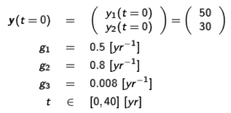
which is essentially the same as \( \dot{\textbf{y}}(t)=\textbf{f}(t, \textbf{y}(t)) \) using the parameters
import matplotlib.pyplot as plt
import scipy
import numpy as np
g1 = 0.5
g2 = 0.8
g3 = 0.008
def f(t, y):
return np.array([
g1 * y[0] - g3 * y[0] * y[1],
-g2 * y[1] + g3 * y[0] * y[1]
])
if __name__ == '__main__':
sol = scipy.integrate.solve_ivp(f, [0, 40], (50, 30), t_eval=np.arange(0, 40, 0.5))
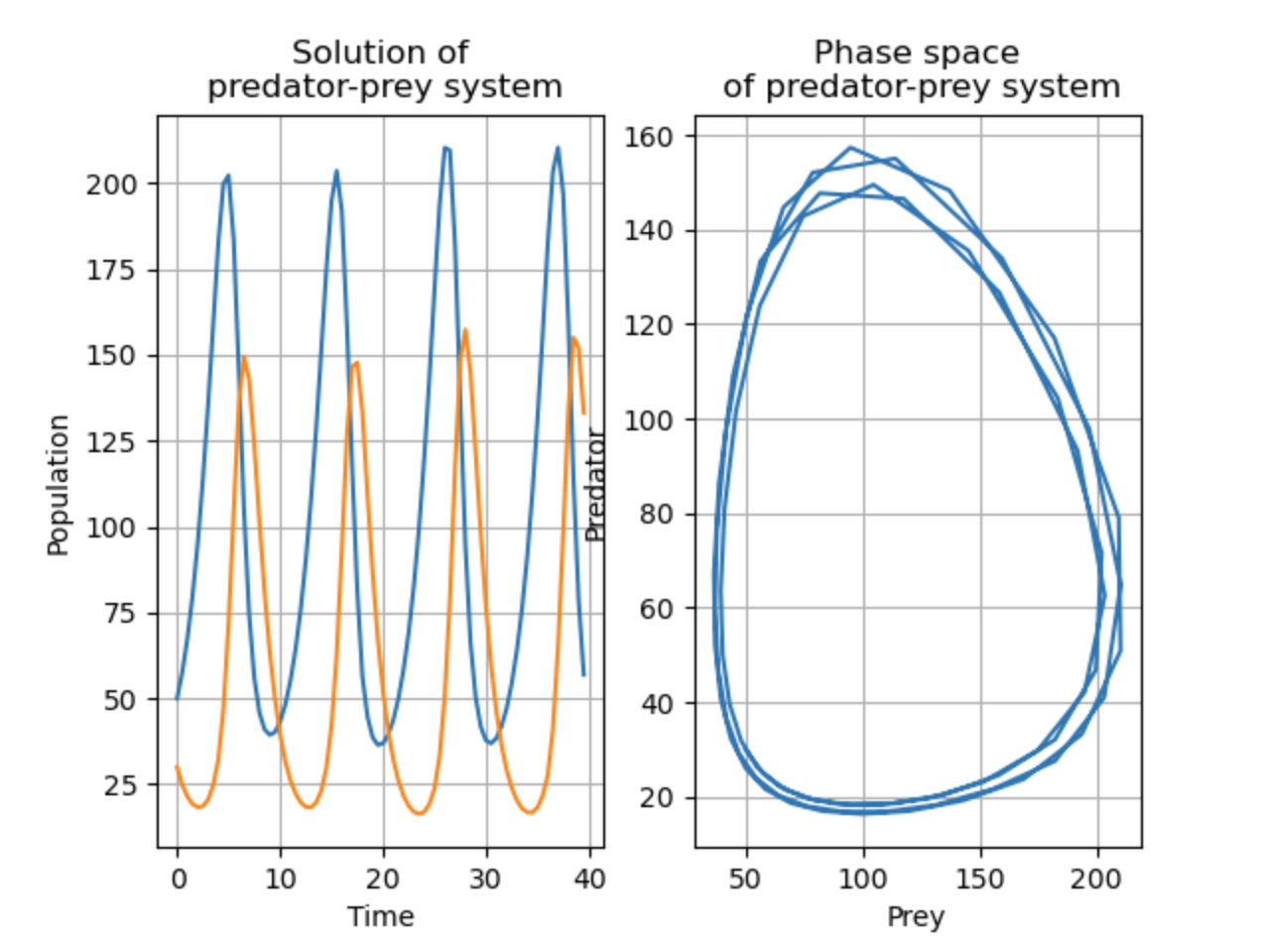
ax1 = plt.subplot(1, 2, 1)
ax1.plot(sol.t, sol.y[0], label='Prey')
ax1.plot(sol.t, sol.y[1], label='Predator')
ax1.set_xlabel('Time')
ax1.set_ylabel('Population')
ax1.set_title('Solution of predator-prey system')
ax1.grid(True)
# Plot phase space
ax2 = plt.subplot(1, 2, 2)
ax2.plot(sol.y[0], sol.y[1])
ax2.set_xlabel('Prey')
ax2.set_ylabel('Predator')
ax2.set_title('Phase space of predator-prey system')
ax2.grid(True)
plt.show()
Resulting in:
Gravity
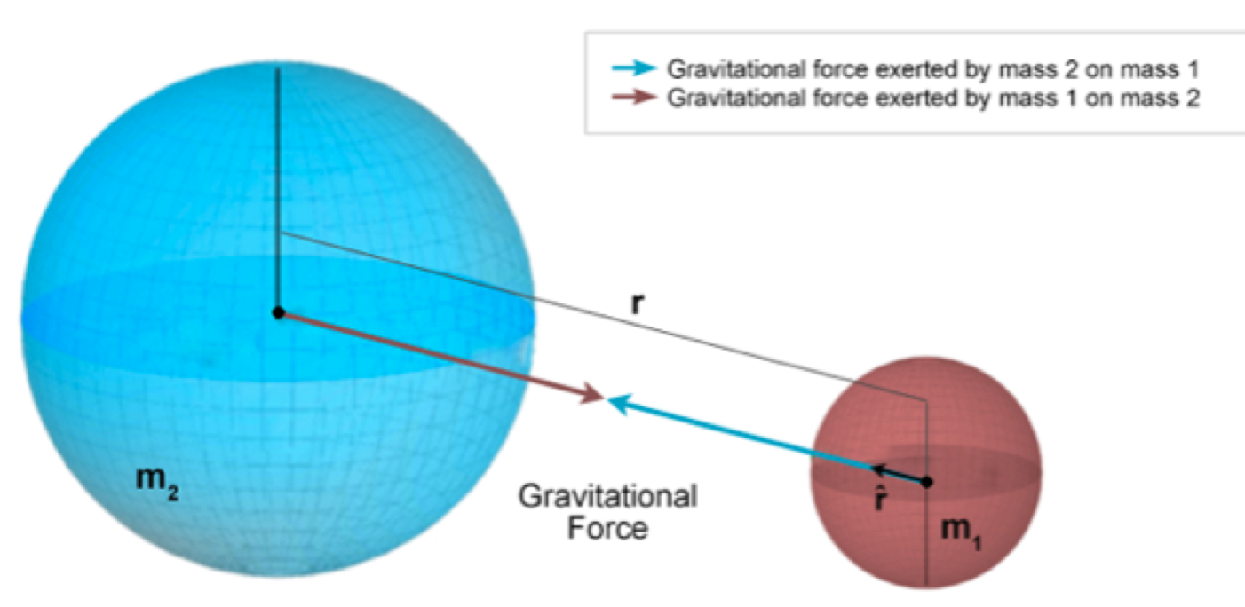
Earth's gravity is modeled by the following differential equation:
\[ \textbf{r}''=-GM\cdot\frac{1}{|\textbf{r}|^2}\cdot\frac{\textbf{r}}{|\textbf{r}|}=-GM\cdot\frac{\textbf{r}}{|\textbf{r}|^3} \]
where \(G\) is the gravitational constant, \(M\) is the mass of the Earth, and \(\textbf{r}\) is the position vector of the satellite. Thus, we have a system of three coupled ODEs:
\[ \begin{pmatrix}x''\\y''\\z''\\ \end{pmatrix} = \begin{pmatrix} -GM\cdot\frac{x}{\sqrt{x^2+y^2+z^2}^3}\\ -GM\cdot\frac{y}{\sqrt{x^2+y^2+z^2}^3}\\ -GM\cdot\frac{z}{\sqrt{x^2+y^2+z^2}^3}\\ \end{pmatrix} \]
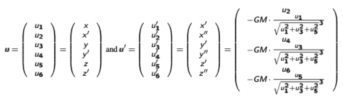
We reduce the system to a system of ODEs of first order by introducing the vector u:
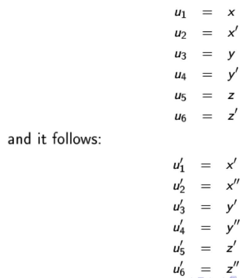
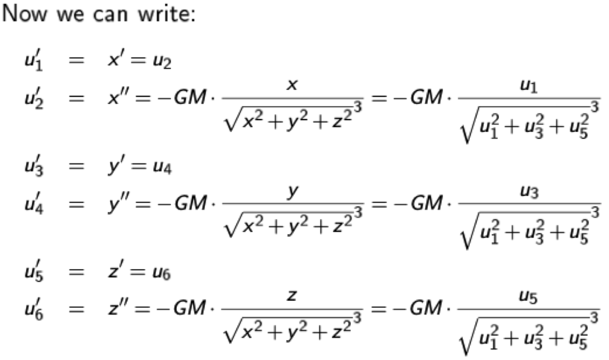
resulting in the ODE
import matplotlib.pyplot as plt
import numpy as np
import scipy
G = 6.67430e-11 # Gravitational constant in m^3 kg^-1 s^-2
M = 1.98892e30 # Mass of the Sun in kg
# Gravitation ODE
def f(t, u):
return np.array([
u[1],
-G * M * u[0] / np.linalg.norm([u[0], u[2], u[4]]) ** 3,
u[3],
-G * M * u[2] / np.linalg.norm([u[0], u[2], u[4]]) ** 3,
u[5],
-G * M * u[4] / np.linalg.norm([u[0], u[2], u[4]]) ** 3
])
if __name__ == '__main__':
# Initial conditions
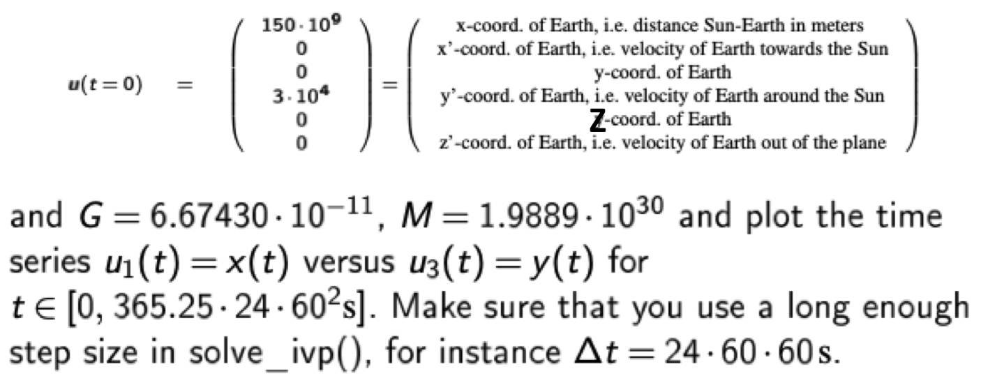
u0 = np.array([150e9, 0, 0, 3e4, 0, 0])
# Solve ODE
step_size = 24 * 60 * 60 # 1 day
t_max = 365.25 * 24 * 60 * 60 # 1 year
sol = scipy.integrate.solve_ivp(f, [0, t_max], u0, t_eval=np.arange(0, t_max, step_size))
# Plot solution
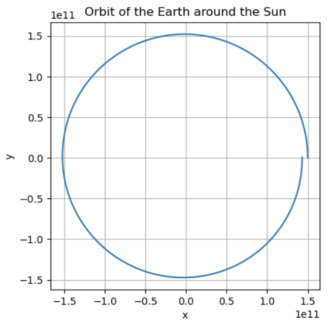
plt.plot(sol.y[0], sol.y[2])
plt.xlabel('x')
plt.ylabel('y')
plt.title('Orbit of the Earth around the Sun')
plt.grid(True)
plt.gca().set_aspect('equal', adjustable='box')
plt.show()