ODEs
Solving a single ODE
Solving a system of ODEs
using solve_ivp
from scipy.integrate:
scipy.integrate.solve_ivp(fun, t_span, y0,
                          method='RK45', t_eval=None, dense_output=False, events=None,
                          vectorized=False, args=None, **options)
Example for \(y' = -y\) for \( t\in [-5,5] \) and \(y_0 = y(-5) = e^5\):
import matplotlib.pyplot as plt
import scipy
import numpy as np

t_span = [-5, 5]
y_0 = [np.exp(5)]

if __name__ == "__main__":
    solution = scipy.integrate.solve_ivp(
        lambda t, y: -y,
        t_span, y_0, t_eval=np.arange(-5, 5, 0.1)
    )

    plt.plot(solution.t, solution.y[0])
    plt.show()
System of ODEs
Predator-Prey model
Solving a system of ODEs
using solve_ivp
from scipy.integrate.
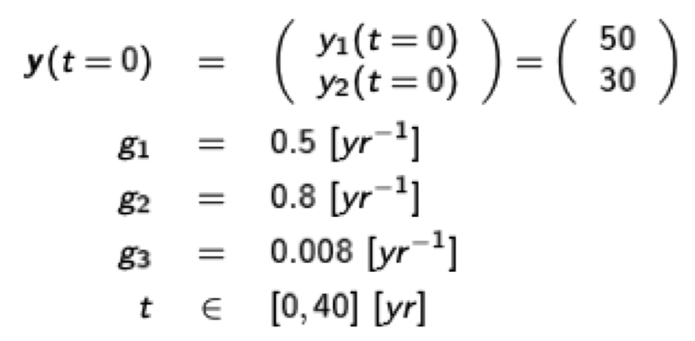
Example for the two-dimensional Lotka-Volterra (predator-prey) equations:
\[\begin{pmatrix}\frac{dy_1}{dt} \\ \frac{dy_2}{dt} \end{pmatrix}=\begin{pmatrix} g_1y_1-g_3y_1y_2 \\ -g_2y_2 + g_3y_1y_2 \end{pmatrix} \]
which is essentially the same as \( \dot{\textbf{y}}(t)=\textbf{f}(t, \textbf{y}(t)) \) using the parameters
import matplotlib.pyplot as plt
import scipy
import numpy as np
g1 = 0.5
g2 = 0.8
g3 = 0.008
def f(t, y):
return np.array([
g1 * y[0] - g3 * y[0] * y[1],
-g2 * y[1] + g3 * y[0] * y[1]
])
if __name__ == '__main__':
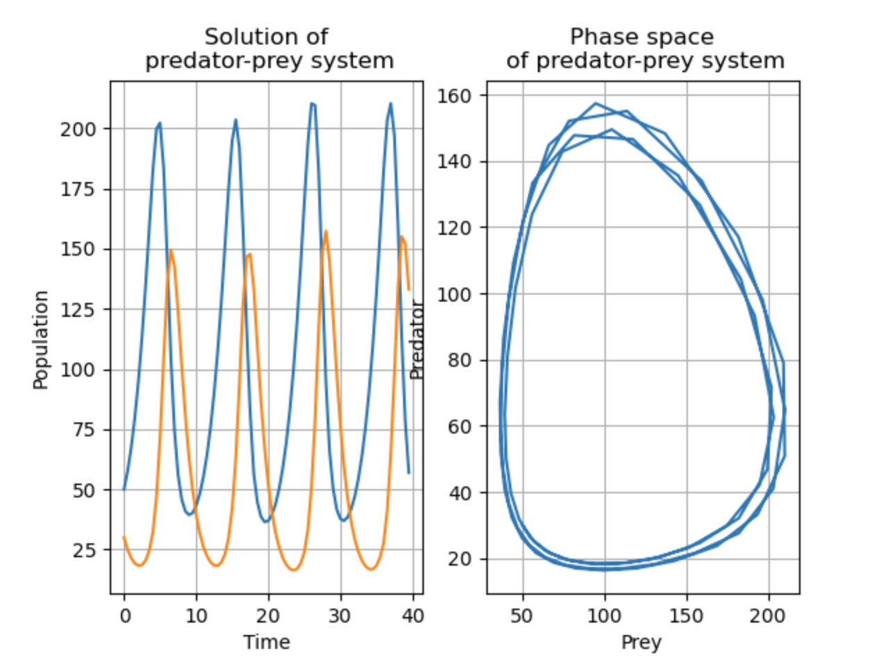
sol = scipy.integrate.solve_ivp(f, [0, 40], (50, 30), t_eval=np.arange(0, 40, 0.5))
ax1 = plt.subplot(1, 2, 1)
ax1.plot(sol.t, sol.y[0], label='Prey')
ax1.plot(sol.t, sol.y[1], label='Predator')
ax1.set_xlabel('Time')
ax1.set_ylabel('Population')
ax1.set_title('Solution of predator-prey system')
ax1.grid(True)
# Plot phase space
ax2 = plt.subplot(1, 2, 2)
ax2.plot(sol.y[0], sol.y[1])
ax2.set_xlabel('Prey')
ax2.set_ylabel('Predator')
ax2.set_title('Phase space of predator-prey system')
ax2.grid(True)
plt.show()
Resulting in:
Gravity
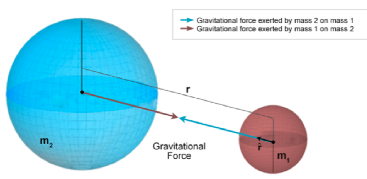
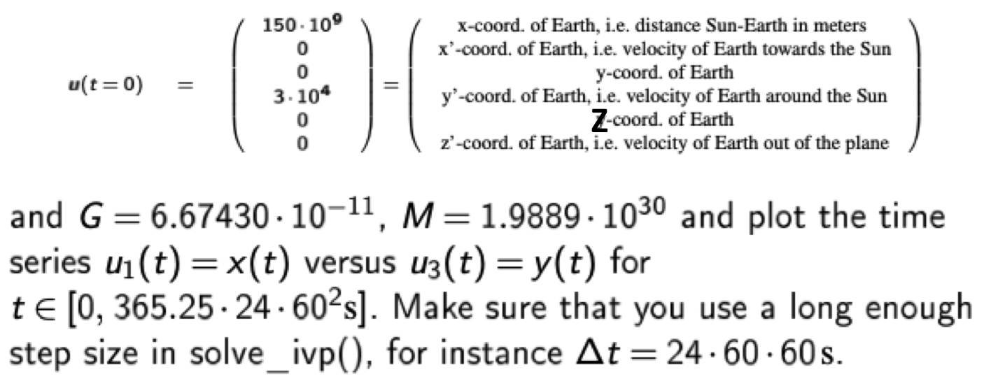
Earth's gravity is modeled by the following differential equation:
\[ \textbf{r}''=-GM\cdot\frac{1}{|\textbf{r}|^2}\cdot\frac{\textbf{r}}{|\textbf{r}|}=-GM\cdot\frac{\textbf{r}}{|\textbf{r}|^3} \]
where \(G\) is the gravitational constant, \(M\) is the mass of the Earth, and \(\textbf{r}\) is the position vector of the satellite. Thus, we have a system of three coupled ODEs:
\[ \begin{pmatrix}x''\\y''\\z''\\ \end{pmatrix} = \begin{pmatrix} -GM\cdot\frac{x}{\sqrt{x^2+y^2+z^2}^3}\\ -GM\cdot\frac{y}{\sqrt{x^2+y^2+z^2}^3}\\ -GM\cdot\frac{z}{\sqrt{x^2+y^2+z^2}^3}\\ \end{pmatrix} \]
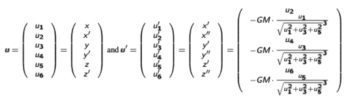
We reduce the system to a system of ODEs of first order by introducing the vector u:
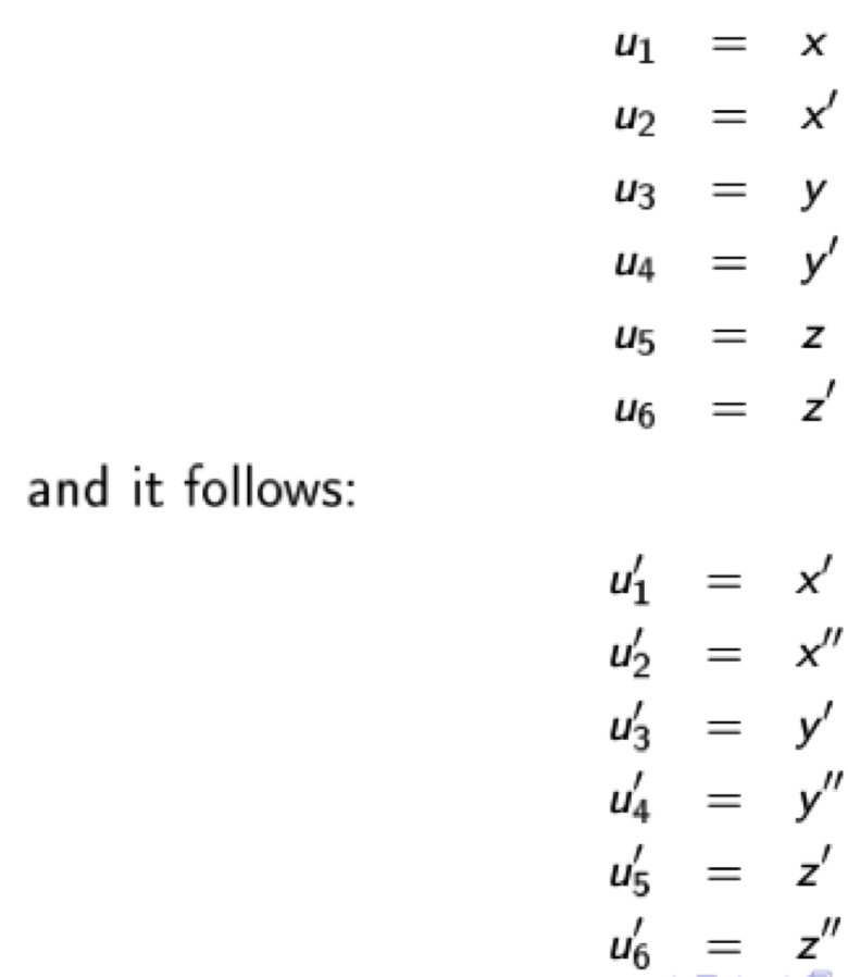
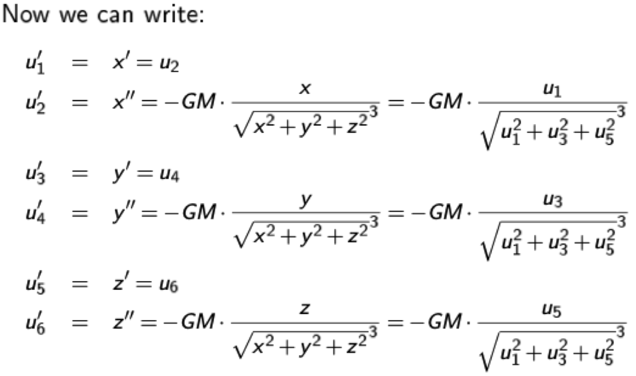
resulting in the ODE
import matplotlib.pyplot as plt
import numpy as np
import scipy
G = 6.67430e-11 # Gravitational constant in m^3 kg^-1 s^-2
M = 1.98892e30 # Mass of the Sun in kg
# Gravitation ODE
def f(t, u):
return np.array([
u[1],
-G * M * u[0] / np.linalg.norm([u[0], u[2], u[4]]) ** 3,
u[3],
-G * M * u[2] / np.linalg.norm([u[0], u[2], u[4]]) ** 3,
u[5],
-G * M * u[4] / np.linalg.norm([u[0], u[2], u[4]]) ** 3
])
if __name__ == '__main__':
# Initial conditions
u0 = np.array([150e9, 0, 0, 3e4, 0, 0])
# Solve ODE
step_size = 24 * 60 * 60 # 1 day
t_max = 365.25 * 24 * 60 * 60 # 1 year
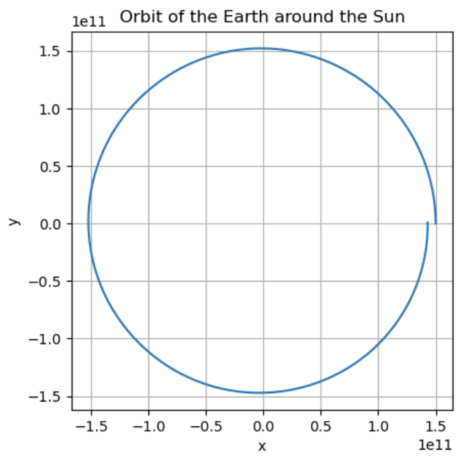
sol = scipy.integrate.solve_ivp(f, [0, t_max], u0, t_eval=np.arange(0, t_max, step_size))
# Plot solution
plt.plot(sol.y[0], sol.y[2])
plt.xlabel('x')
plt.ylabel('y')
plt.title('Orbit of the Earth around the Sun')
plt.grid(True)
plt.gca().set_aspect('equal', adjustable='box')
plt.show()
Matrix Transformations
Translation
A translation moves all the points of a shape by the same amount in the x and y directions. The amount to move in the x direction is called tx and the amount to move in the y direction is called ty. The translation matrix is:
\[ \begin{bmatrix} 1 & 0 & tx \\ 0 & 1 & ty \\ 0 & 0 & 1 \end{bmatrix} \cdot \begin{bmatrix} x \\ y \\ 1 \end{bmatrix} = \begin{bmatrix} x + tx \\ y + ty \\ 1 \end{bmatrix} \]
Rotation
Rotation is a transformation that rotates a shape around a fixed point. The fixed point is called the center of rotation. The amount to rotate is called θ (theta). The rotation matrix is:
\[ \begin{bmatrix} \cos(\theta) & -\sin(\theta) & 0 \\ \sin(\theta) & \cos(\theta) & 0 \\ 0 & 0 & 1 \end{bmatrix} \cdot \begin{bmatrix} x \\ y \\ 1 \end{bmatrix} = \begin{bmatrix} x \cos(\theta) - y \sin(\theta) \\ x \sin(\theta) + y \cos(\theta) \\ 1 \end{bmatrix} \]
import numpy as np

def translate_and_rotate_around_point(p_old, a, b, phi):
    translation_matrix = np.array([
        [1, 0, a],
        [0, 1, b],
        [0, 0, 1]
    ])

    rotation_matrix = np.array([
        [np.cos(phi), -np.sin(phi), 0],
        [np.sin(phi), np.cos(phi), 0],
        [0, 0, 1]
    ])

    return (translation_matrix @ rotation_matrix @ np.linalg.inv(translation_matrix)) @ p_old
Scaling
Scaling is a transformation that changes the size of a shape. The amount to scale in the x direction is called sx and the amount to scale in the y direction is called sy. The scaling matrix is:
\[ \begin{bmatrix} sx & 0 & 0 \\ 0 & sy & 0 \\ 0 & 0 & 1 \end{bmatrix} \cdot \begin{bmatrix} x \\ y \\ 1 \end{bmatrix} = \begin{bmatrix} sx \cdot x \\ sy \cdot y \\ 1 \end{bmatrix} \]
Plot animation
Using the matplotlib.animation
and FuncAnimation
module, we can create animations of our plots:
class matplotlib.animation.FuncAnimation(
    fig, func,
    frames=None, init_func=None, fargs=None, save_count=None, *, cache_frame_data=True, **kwargs
)
Earth rotation around sun
import numpy as np
import matplotlib.pyplot as plt
from matplotlib.animation import FuncAnimation


def rotate_around_point(p_old, a, b, phi):
    translation_matrix = np.array([
        [1, 0, a],
        [0, 1, b],
        [0, 0, 1]
    ])

    rotation_matrix = np.array([
        [np.cos(phi), -np.sin(phi), 0],
        [np.sin(phi), np.cos(phi), 0],
        [0, 0, 1]
    ])

    return (translation_matrix @ rotation_matrix @ np.linalg.inv(translation_matrix)) @ p_old


if __name__ == '__main__':
    # start coordinates of earth
    earth = np.array([5, 0, 1])

    # coordinates of the sun
    sun = np.array([0, 0, 1])

    n_per_day = 5
    n_days = 365
    n = n_days * n_per_day  # number of iterations
    phi_rotate = (np.pi * 2) / n  # angular velocity earth - sun

    # Earths orbit with respect to time
    earth_coordinates = [earth]
    for i in range(n):
        earth_coordinates.append(
            rotate_around_point(earth_coordinates[-1], sun[0], sun[1], phi_rotate)
        )

    fig, ax = plt.subplots()
    plt.plot(sun[0], sun[1], '*b')
    ln, = plt.plot([], [], 'or')


    def init():
        ax.axis([-8, 8, -8, 8])
        ax.set_aspect('equal', 'box')
        return ln,


    def update(frame):
        ln.set_data(earth_coordinates[frame][0], earth_coordinates[frame][1])
        return ln,


    ani = FuncAnimation(fig, update, frames=n, init_func=init, interval=10)
    plt.show()
Image Processing
Idea: Replace each pixel value with a function of its neighborhood using a filter kernel (e.g. a 3x3 matrix).
Standard Filters
Average
Replace each pixel with the average of its neighborhood using a filter kernel like
\[ \frac{1}{9} \cdot \begin{pmatrix} 1 & 1 & 1 \\ 1 & 1 & 1 \\ 1 & 1 & 1 \end{pmatrix} \]
Sharpen
To sharpen the original image, add the subtraction of the blurred image from the original image to the original image.
\[ \begin{pmatrix} 0 & 0 & 0 \\ 0 & 1 & 0 \\ 0 & 0 & 0 \end{pmatrix} - \frac{1}{9} \cdot \begin{pmatrix} 1 & 1 & 1 \\ 1 & 1 & 1 \\ 1 & 1 & 1 \end{pmatrix} + \begin{pmatrix} 0 & 0 & 0 \\ 0 & 1 & 0 \\ 0 & 0 & 0 \end{pmatrix} = \begin{pmatrix} -\frac{1}{9} & -\frac{1}{9} & -\frac{1}{9} \\ -\frac{1}{9} & 2 - \frac{1}{9} & -\frac{1}{9} \\ -\frac{1}{9} & -\frac{1}{9} & -\frac{1}{9} \end{pmatrix} \]
Gaussian Blur
Weight neighboring pixels by a Gaussian distribution
\[
G_\sigma = \frac{1}{2\pi\sigma^2} \cdot e^{-\frac{x^2+y^2}{2\sigma^2}}
\]
e.g. for a 5x5 kernel with \( \sigma = 1 \)
\[ \begin{pmatrix} 0.003 & 0.013 & 0.022 & 0.013 & 0.003 \\ 0.013 & 0.059 & 0.097 & 0.059 & 0.013 \\ 0.022 & 0.097 & 0.159 & 0.097 & 0.022 \\ 0.013 & 0.059 & 0.097 & 0.059 & 0.013 \\ 0.003 & 0.013 & 0.022 & 0.013 & 0.003 \end{pmatrix} \]
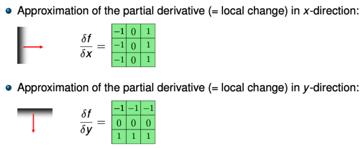
Gradient filters / Edge detection
The gradient \(\mathrm{grad}(f) = \begin{pmatrix} \frac{\partial f}{\partial x} & \frac{\partial f}{\partial y} \end{pmatrix}^T\) measures the rate of change of function \(f\) in the \(x\) and \(y\) directions. Hence, the magnitude \(|\mathrm{grad}(f)|\) measures how quickly the function changes.
Applying a filter using convolution
import numpy as np

def convolve(image, kernel):
    # Pad image with zeros to avoid boundary effects
    padded_image = np.pad(image, kernel.shape[0] // 2, mode='constant')
    output = np.zeros_like(image)

    # Loop over every pixel of the image
    for x in range(image.shape[1]):
        for y in range(image.shape[0]):
            output[y, x] = (kernel * padded_image[y:y + kernel.shape[0], x:x + kernel.shape[1]]).sum()
    return output

kernel = np.ones((3, 3)) / 9
filtered_image = convolve(my_image, kernel)
Naive Bayes
Model assumption: Independence of features (No correlation between features), e.g. \(P(\text{Rain}\wedge\text{Hot})=P(\text{Rain})\cdot P(\text{Hot})\).
Events are described by a feature vector \(\mathbf{X}\) of length \(n\), where \(X_i\) is the value of the \(i\)-th feature. Outcome is described by a prediction-variable \(Y\in \text{{0, 1}}\).
Estimations: \[P(X|Y=0) := \prod_{i=1}^n P(X_i | Y=0)\] \[P(X|Y=1) := \prod_{i=1}^n P(X_i | Y=1)\] \[P(Y=0 | X) := \frac{P(X|Y) \cdot P(Y=0)}{P(X)} \] \[P(Y=1 | X) := \frac{P(X|Y) \cdot P(Y=1)}{P(X)}\]
If \(P(Y = 0 | X)\) > \(P(Y = 1 | X)\), then \(Y = 0\), otherwise predict \(Y = 1\).
Laplace Smoothing
If a feature value is not present in the training set, then the probability will be zero. To avoid this, we can use Laplace smoothing, which adds a small constant \(\alpha = 1\) to the numerator and \(2\alpha\) to the denominator.
Classification Example
from load_data import loadData


def train(training_mails, training_labels):
    """
    Train the model on the training data.
    :param training_mails: A matrix where the rows are the mails and the columns are the words.
    :param training_labels: A vector where the i-th entry is the label of the i-th mail. 1 means spam, 0 means non-spam.
    """

    spam_mails = training_mails[training_labels == 1]
    non_spam_mails = training_mails[training_labels == 0]

    spam_token_probabilities = spam_mails.sum(axis=0) / spam_mails.sum(axis=(0, 1))
    non_spam_token_probabilities = non_spam_mails.sum(axis=0) / non_spam_mails.sum(axis=(0, 1))

    spam_probability = spam_mails.shape[0] / training_mails.shape[0]
    non_spam_probability = non_spam_mails.shape[0] / training_mails.shape[0]

    return {
        "spam_token_probabilities": spam_token_probabilities,
        "non_spam_token_probabilities": non_spam_token_probabilities,
        "spam_probability": spam_probability,
        "non_spam_probability": non_spam_probability
    }


def calculate_probabilities(testing_mails, token_probabilities):
    """
    Calculate the probability of the mail given it's spam or non-spam.
    :param testing_mails: A matrix where the rows are the mails and the columns are the words.
    :param token_probabilities: The probabilities of the tokens given the mail is spam or non-spam.
    :return: The probability of the mail given it's spam or non-spam.
    """
    return (token_probabilities ** testing_mails).prod(axis=1)


def test(testing_mails, testing_labels, model):
    """
    Test the model on the testing data.
    :param testing_mails: A matrix where the rows are the mails and the columns are the words.
    :param testing_labels: A vector where the i-th entry is the label of the i-th mail. 1 means spam, 0 means non-spam.
    :return: The accuracy of the model.
    """

    spam_token_probabilities, non_spam_token_probabilities, spam_probability, non_spam_probability = model.values()

    spam_probability = calculate_probabilities(testing_mails, spam_token_probabilities) * spam_probability
    non_spam_probability = calculate_probabilities(testing_mails, non_spam_token_probabilities) * non_spam_probability

    predicted_labels = (spam_probability > non_spam_probability).astype(int)
    accuracy = (predicted_labels == testing_labels).sum() / len(testing_labels)

    print(f"Predicted labels: {predicted_labels}, actual labels: {testing_labels}")
    print("Acccuracy: %.2f%% => Error-Rate: %.2f%%" % (accuracy * 100, (1 - accuracy) * 100))

    return accuracy


if __name__ == "__main__":
    loaded_data = loadData()
    model = train(
        training_mails=loaded_data['trainMatrixEx1'],
        training_labels=loaded_data['trainLabelsEx1']
    )

    test(
        testing_mails=loaded_data['testMatrixEx1'],
        testing_labels=loaded_data['testLabelsEx1'],
        model=model
    )
Clustering
k-means algorithm

K-means clustering is an unsupervised machine learning algorithm that divides a dataset into a specified number of clusters (k). The goal is to group similar data points together within a cluster and separate dissimilar data points into different clusters.
Here's a simple example of how the algorithm works:
- Choose the number of clusters (k) and randomly select k data points as the initial centroids for each cluster.
- Calculate the distance between each data point and the centroids.
- Assign each data point to the cluster with the nearest centroid.
- Recalculate the centroid for each cluster by taking the mean of all the data points in the cluster.
- Repeat steps 2-4 until the centroids no longer move or the maximum number of iterations is reached.
import numpy as np
import matplotlib.pyplot as plt
from sklearn.datasets import make_blobs
from sklearn.metrics import silhouette_score


def k_means(X, k, max_iters=100):
    # Initialize centroids randomly
    centroids = X[np.random.choice(len(X), k, replace=False)]

    for _ in range(max_iters):
        # Calculate distances between each data point and each centroid
        distances = np.sqrt(((X - centroids[:, np.newaxis]) ** 2).sum(axis=2))

        # Assign each data point to the cluster with the nearest centroid
        clusters = np.argmin(distances, axis=0)

        # Recalculate the centroid for each cluster
        centroids = np.array([X[clusters == i].mean(axis=0) for i in range(k)])

    return centroids, clusters


if __name__ == '__main__':
    # Generate some random data
    X, y = make_blobs(n_samples=1000, centers=3, n_features=2, random_state=42)

    # Plot the data
    plt.scatter(X[:, 0], X[:, 1], c=y)
    plt.show()

    found_centroids, clusters = k_means(X, k=3)

    # Plot the data and the clusters
    plt.scatter(X[:, 0], X[:, 1], c=clusters)
    plt.scatter(found_centroids[:, 0], found_centroids[:, 1], marker='x', c='black')
    plt.show()

    print(f"Silhouette score: {silhouette_score(X, clusters)}")
Measuring the quality of clustering
Silhouette coefficient
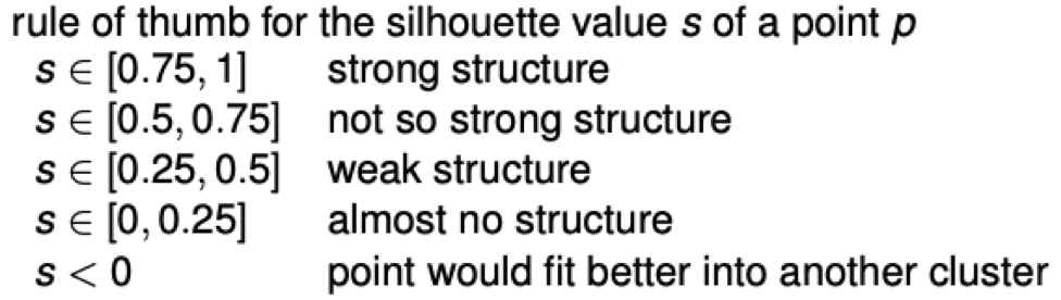
The silhouette coefficient is a measure of how similar an object is to its own cluster (cohesion) compared to other clusters (separation). The silhouette coefficient for a single sample is calculated as follows: \[s_i = \frac{b_i - a_i}{max(a_i, b_i)}\] where \(a_i\) is the mean distance between the sample and all other points in the same cluster, and \(b_i\) is the mean distance between the sample and all other points in the nearest cluster that is not the same as the sample's cluster.
Gaussian Mixture Models
A Gaussian mixture model is a probabilistic model that assumes all the data points are generated from a mixture of a finite number of Gaussian distributions with unknown parameters. Each Gaussian distribution is associated with one of the K components of the model. In the case of multivariate data, a Gaussian mixture model can be thought of as a generalization of the k-means clustering algorithm to incorporate uncertainty in the assignments of points to clusters.
In general, the model represents the probability distribution of the data as a weighted sum of several multivariate Gaussian distributions. The weights associated with each Gaussian reflect the relative importance of that component in the mixture. Given a set of observations, the goal of the Gaussian mixture model is to determine the parameters of the individual Gaussian's and the weights that would best explain the observed data. This is typically done by maximizing the likelihood of the observed data under the model.
import matplotlib.pyplot as plt
from sklearn.datasets import make_blobs
from sklearn.mixture import BayesianGaussianMixture

if __name__ == '__main__':
    # Generate some random data
    X, y = make_blobs(n_samples=1000, centers=3, n_features=2, random_state=42)

    # Plot the data
    plt.scatter(X[:, 0], X[:, 1], c=y)
    plt.show()

    bayesian_gaussian_mixture = BayesianGaussianMixture(n_components=3, random_state=42)
    bayesian_gaussian_mixture.fit(X)
    y_pred = bayesian_gaussian_mixture.predict(X)
    # y_pred is an array of cluster labels for each data point

    # Plot the data and the clusters
    plt.scatter(X[:, 0], X[:, 1], c=y_pred)
    plt.show()
Classification
Nearest Mean Classifier
The nearest mean classifier is a simple classifier that is based on the idea that the mean of the training data for each class is the best estimate of the mean of the data for that class.
- No further knowledge about the structure of the underlying data is required.
- Efficiently computable.
- Outliers can influence the mean and thus the classification.
- The mean is not always a representative point of the data.
- Failure in case of different 'spread of data' (large eigenvalues of the covariance matrix (
np.cov(M.T))).
import numpy as np

def distance(p, q):
    dif = p - q
    return np.linalg.norm(dif, 2)


def classify_nearestmean(A, M, k):
    # classification by nearest mean
    t = M.shape[0]
    r, d = A.shape
    N = r // k

    means = np.zeros((k, d))
    alpha = np.zeros((M.shape[0],))
    for i in range(k):
        T = A[N * i:N * (i + 1)]
        means[i, :] = np.mean(T, axis=0)
    # print(means)
    dist_to_mean = np.zeros((k,))
    for i in range(t):
        P = M[i, :]
        for j in range(k):
            dist_to_mean[j] = distance(P, means[j, :])
        alpha[i] = dist_to_mean.argmin()

    return alpha
Bayes Classifier (based on Gaussian Mixture Model)
Using a distance measure (like the mahalonobis distance) the Bayes classifier can be used to classify data. The distance measure is based on the assumption that the data is distributed according to a Gaussian Mixture Model (GMM).
import numpy as np
import scipy.stats as stats

def classify_gmm(A, M, k):
    """
    Classification by Gaussian mixture model.
    """
    r, d = A.shape
    N = r // k
    means = np.zeros((k, d))
    covariances = np.zeros((k, d, d))

    for i in range(k):
        T = A[N * i:N * (i + 1)]
        means[i, :] = np.mean(T, axis=0)
        covariances[i, :, :] = np.cov(T.T)

    # print(f"means: {means}")
    # print(f"covariances: {covariances}")

    probability_densities = [stats.multivariate_normal.pdf(M, means[j, :], covariances[j, :, :]) for j in range(k)]
    return np.argmax(probability_densities, axis=0)
Principal Component Analysis - PCA
PCA is a dimensionality reduction algorithm. It is used to find the direction of largest variance in high dimensional data and projects it onto a new subspace with equal or fewer dimensions than the original one.
PCA is also used as a tool for visualization, where we can visualize high dimensional data in a lower dimensional space.
Algorithm
The algorithm is as follows:
- Standardize the data.
- Obtain the Eigenvectors and Eigenvalues from the covariance matrix or correlation matrix, or perform Singular Vector Decomposition.
- Sort eigenvalues in descending order and choose the \(k\) eigenvectors that correspond to the \(k\) largest eigenvalues where \(k\) is the number of dimensions of the new feature subspace (\(k\leq d\)).
- Construct the projection matrix \(W\) from the selected \(k\) eigenvectors.
- Transform the original dataset \(X\) via \(W\) to obtain a \(k\)-dimensional feature subspace \(Y\).
import numpy as np
import scipy.linalg as la


def get_eigenvectors(data_matrix, k):
   """
   Calculates the eigenvectors of the data_matrix and returns
   k eigenvectors, sorted descending to their value.
   """
   cov_matrix = np.cov(data_matrix.T)
   n = cov_matrix.shape[0]
   _, eigenvectors = la.eigh(cov_matrix, subset_by_index=[n - k, n - 1])
   return np.flip(eigenvectors, axis=1)


def get_mean(data_matrix):
   """
   Calculates the mean of the data_matrix.
   """
   return np.mean(data_matrix, axis=0)


def compress_pca_vector(vector, mean, eigenvectors):
   p = (vector - mean).reshape(-1, 1)
   return (eigenvectors @ (eigenvectors.T @ p)) + mean.reshape(-1, 1)

if __name__ == '__main__':
   import load_data as ld

    data = ld.load_data()
    print(compress_pca_vector(data['vecTest'], data['mTest'], data['vEigenTest1']))
Skin Cancer Detection
TDS-Algorithm (Total Dermoscopic Score)
\[\mathrm{TDS}=1.3\cdot A+0.1\cdot B+0.5\cdot C+0.5\cdot D\]
- A: Integer value of the number of asymmetry features (0 is symmetric, 1 middle, 2 is asymmetric)
- B: Integer value of the number of border irregularity features (0 to 8 indicating the presence of border irregularities in 8 regions)
- C: Integer value indicating the presence of one to six specific colors (1 to 6)
- D: Integer value indicating presence of one to five distinct structures or textures (1 to 5)
| Evaluation | TDS Score |
|---|---|
| Benign | < 4.75 |
| Suspicious | 4.75 to 5.45 |
| Malignant | > 5.45 |
Process
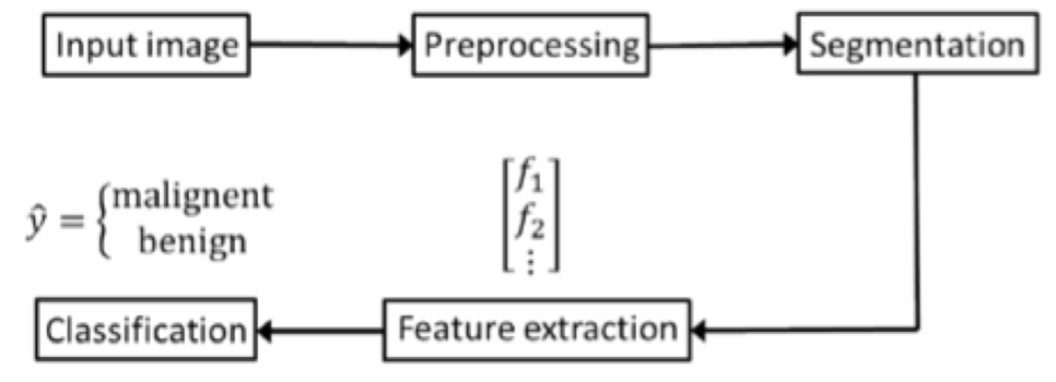
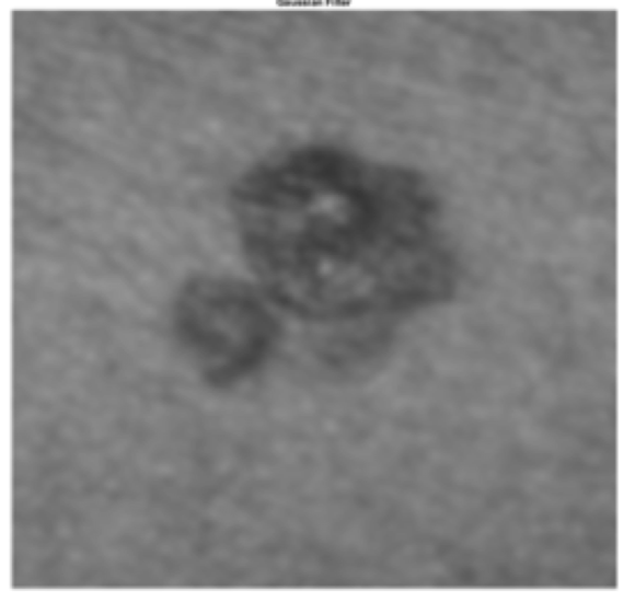
1. Preprocessing
- Grayscale
- Crop-in by a factor
- Apply a Gaussian blur (with sigma=5)
Output
2. Segmentation
- Using Otsu's method to turn the filtered grey-scale image into a binary image
- fill the holes in the image.
- Find the contours of the shape using
cv2.findContours
Output

3. Feature Extraction
- Calculate the centroid and bounding box
- Calculate color score
- For each pixel within the lesion area, the euclidean distance from 6 RGB values is calculated
- For each color, the count is increased if the pixel is closest to it
- The end result is a vector of 6 values, each representing the count of pixels closest to the color, which will be divided by the total number of pixels
- For each color with a value greater than 0.01, a point is given to the TDS C score
- Calculate the variance of the RGB values: \[variance=\sigma^2=\frac{1}{n}\sum_{i=1}^{n}(x_i-\bar{x})^2\] where \(x_i\) is the RGB value of the pixel, \(\bar{x}\) is the mean of the RGB values \(\bar{x}=\frac{1}{n}\sum_{i=1}^n x_i\), and \(n\) is the number of pixels
- Calculate the asymmetry score
- The centroid is calculated
- For each degree out of 360 degrees, the radii in polar coordinates are calculated
- For each radii, the length of the symmetric radii is calculated and for pairs of which the difference of distances is less than 10%, a point is given
- The sum of points is the \(\mathrm{SFA}_i\) (Score For Axis) score.
- The radius with the maximum \(\mathrm{SFA}\) score is defined as the major axis of symmetry.
- The asymmetry score is calculated as follows:
| Evaluation | Asymmetry score |
|---|---|
| major axis \(\geq 140\) and minor axis \(\geq 140\) | Symmetric across both axis ==> 0 |
| major axis \(\geq 140\) and minor axis \(\lt 140\) | symmetric across one axis ==> 1 |
| major axis \(\lt 140\) and minor axis \(\lt 140\) | asymmetric ==> 2 |
PDEs
Plot a surface
import matplotlib.pyplot as plt
import numpy as np


def f1(x, y):
    return x ** 2 - y ** 2


if __name__ == '__main__':
    x = np.linspace(-np.pi, np.pi, 100)
    y = np.linspace(-np.pi, np.pi, 100)
    X, Y = np.meshgrid(x, y)
    Z = f1(X, Y)
    fig = plt.figure()
    ax = fig.add_subplot(projection='3d')
    ax.plot_surface(X, Y, Z, cmap='viridis', edgecolor='none', linewidth=0.5)
    plt.xlabel('x')
    plt.ylabel('y')
    plt.title('z = f1(x, y)')
    plt.show()
Partial derivatives of first order
Given a function \(f: \mathbb{R}^n \rightarrow \mathbb{R}\), the partial derivative of \(f\) with respect to \( x_i\) is defined as
\[ \frac{\partial f}{\partial x_i} = \lim_{\Delta y \rightarrow 0} \frac{f(x_1, \ldots, x_i + \Delta y, \ldots, x_n) - f(x_1, \ldots, x_i, \ldots, x_n)}{\Delta y}. \]
The gradient of the function \(f\) is defined as
\[ \mathrm{grad}(f) = \nabla f = \left( \frac{\partial f}{\partial x_1}, \ldots, \frac{\partial f}{\partial x_n} \right)^T \]
Partial derivatives of higher order
Schwartz's theorem
Let \(f: \mathbb{R}^n \rightarrow \mathbb{R}\) be a function. If the mixed partial derivatives exist and are continuous at a point \(x_0\in\mathbb{R}^n\), then they are equal at \(x_0\) regardless of the order in which they are taken.
Laplacian
Let \(f: \mathbb{R}^n \rightarrow \mathbb{R}\) be a function. The Laplacian of \(f\) is defined as
\[ \Delta f = \nabla^2 f = \sum_{i=1}^n \frac{\partial^2 f}{\partial x_i^2} = \left( \frac{\partial^2 f}{\partial x_1^2}+\ldots+\frac{\partial^2 f}{\partial x_n^2} \right) \]
Fourier series
Let \(f: \mathbb{R} \rightarrow \mathbb{R}\) be a periodic continuous function with angular frequency \(\omega_0\) and period \(T = 2\pi\div\omega_0\). The Fourier series of \(f\) is defined as
\[ f(x) = \frac{a_0}{2} + \sum_{n=1}^\infty \left( a_n \cos(n\omega_0 x) + b_n \sin(n\omega_0 x) \right) \]
where
\[ \begin{matrix} a_0 = \frac{2}{T} \int_{(T)} f(x)\ dx \\ a_n = \frac{2}{T} \int_{(T)} f(x) \cos(n\omega_0 x)\ dx \\ b_n = \frac{2}{T} \int_{(T)} f(x) \sin(n\omega_0 x)\ dx \end{matrix} \]
(Integration over period T)
Partial Differential Equation
Linear, homogenous PDE of first order
If the coefficients \(a = a(x, y) \) and \(b = b(x, y) \) are continuously differentiable functions \(a: D \subset\mathbb{R}^2\rightarrow\mathbb{R} \) and \(b: D \subset\mathbb{R}^2\rightarrow\mathbb{R} \), then the PDE for \(u = u(x, y) \)
\[ a(x,y)\cdot u_x+b(x,y)\cdot u_y=0 \]
is a linear homogenous PDE of first order. Homogenous means that the right side of the PDE vanishes (is zero).
Superposition principle
If \(u_1 = u_1(x, y) \) and \(u_2 = u_2(x, y) \) are solutions of a linear, homogenous PDE, then \(u_1 + u_2 \) is also a solution.
Linear PDE of second order
notation: \( f_{xy} = \frac{\partial^2 f}{\partial x \partial y} \) is a mixed partial derivative
Consider the continuously differentiable functions \(a,b,c,d,e,f,g: D \subset\mathbb{R}^2\rightarrow\mathbb{R} \). The PDE for \(u = u(x, y) \)
\[ a(x,y)\cdot u_{xx}+2b(x,y)\cdot u_{xy}+c(x,y)\cdot u_{yy}=d(x,y)\cdot u_x+e(x,y)\cdot u_y+f(x,y)\cdot u+g(x,y) \]
is a linear PDE of second order (assuming \(u_{xy}=u_{yx} \).
Computational Fluid Dynamics
Governing Equations
The mass conservation equation
The mass conservation equation is given by
\[ \frac{\partial \rho}{\partial t} + \nabla \cdot (\rho \vec{u}) = 0 \]
where \(\rho\) is the density of the fluid and \(\vec{u}\) is the velocity vector. For an incompressible fluid, the density is constant, the equation simplifies to
\[ \nabla \cdot \vec{u} = 0 \]
The momentum conservation equation
The momentum conservation equation is given by
\[ \frac{\partial \rho u}{\partial t} + \nabla \cdot (\rho \vec{u} u) = \nabla\cdot(\mu\nabla u)-\frac{\partial p}{\partial x}+S_{Mx} \] \[ \frac{\partial \rho v}{\partial t} + \nabla \cdot (\rho \vec{u} v) = \nabla\cdot(\mu\nabla v)-\frac{\partial p}{\partial y}+S_{My} \] \[ \frac{\partial \rho w}{\partial t} + \nabla \cdot (\rho \vec{u} w) = \nabla\cdot(\mu\nabla w)-\frac{\partial p}{\partial z}+S_{Mz} \]
where \(\rho\) is the density of the fluid, \(\vec{u} = (u, v, w)\) is the velocity vector, \(\mu\) is the dynamic viscosity of the fluid, \(p\) is the pressure of the fluid, and \(S_{Mx}\), \(S_{My}\), and \(S_{Mz}\) are the source terms which describe the effects of body forces such as the centrifugal force.
The energy conservation equation
The energy conservation equation is given by
\[ \frac{\partial \rho i}{\partial t} + \nabla \cdot (\rho \vec{u} i) = \nabla\cdot(k\nabla T)-p\nabla\cdot\vec{u}+S_{\mathrm{Dis}} \]
where \(i\) is the spedific internal energy of the fluid, \(k\) is the thermal conductivity of the fluid, \(T\) is the temperature of the fluid, and \(S_{\mathrm{Dis}}\) is the source term which describes the effects of body forces
Equations of State
\(p = p(\rho, T)\) and \(i = i(\rho, T)\)
Task reference list
- Task 1: Solve a system of ODEs
- Task 2: Matrix transformations and plot animation
- Task 3: Image Processing
- Task 4: Naive Bayes
- Task 5: Clustering
- Task 6: Classification
- Task 7: PCA
- Task 8: Skin Cancer Detection
- Task 9: PDEs